IS-LM Model

Before I boil down into this fascinating model which was the precursor to the macroeconomic diagrams and models that all highschool economic students are familiar with (the AD-AS model), here are a couple of points that will give a good indication about this article to all the readers reading this.

1. This is beyond high-school economics; therefore, if you are a non-economics student, it is best you read some of the other articles, i.e. the Themes' ones. Or, if you are intrigued to understand this highly intuitive and fundamental model, do feel free to ask any point of clarification in the "ask your doubts!" tab.

2. There will be no direct application here. Even though this may be perceived as straying away from the mission of this site, the purpose behind this article is to present the model which was what facilitated the creation of the major macroeconomic models that are applied in many areas (some of which are in the Themes section itself).

Okay now that the "disclaimer" is over, let's dig in.

There are two aspects of this model: the macroeconomic product market/economy and the money market. It is a situation of general equilibrium (because there is equilibrium in more than one market, at the same time).

So let's start with the macroeconomy! What is considered equilibrium there? Well, in this article, we will be utilizing the work of John Maynard Keynes (since it was actually the interpretation of his book that led to the construction of this model). But before we look at Keynesian Economics, all high school economics students will know about the circular flow of income models (in a closed and open economy). An important assumption is that the IS curve follows the CLOSED ECONOMY. Again, one may exclaim the fact that this is not applicable in the real world, and again, the purpose of this model is not to be applied but rather, understood (because it is a fundamental model, which has been extended into applicable models).

When talking about the closed economy, we know that aggregate income is equal to aggregate expenditure which is equal to aggregate output and this is the equilibrium of income/output and expenditure. The curve, which I am about to display, showcases (the aforementioned) equilibrium at every single point on the curve.

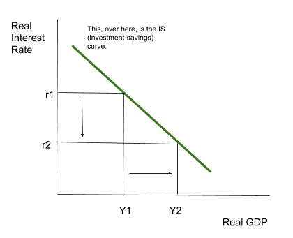
So, the graph that I made, shows a curve (green) that represents income-expenditure equilibrium is known as the investment-savings curve. Even though the graph is linear in nature, one may have an assortment of questions, right from "why is it called investment-savings curve" to "why do real interest rates and real GDP have that relationship".

Let's answer it all :). The best way to do this would be to start off with the assumption on hand -> aggregate expenditure is equal to aggregate income. So getting mathematical here, what are the functions that we have?

Aggregate Income = Y

Aggregate Expenditure = C (consumption) + G (govt. expenditure) + I (investment/firm expenditure)

[for all the high-school economics students, remember this is a model in the closed economy, so no net exports].

So, aggregate income = aggregate expenditure

-> Y = C(Y-t) + G + I(r)

(the brackets are not parenthesis, they are functional notation, for example consumption is a function of disposable income (Y-t). Also, t = taxes and r = interest rate (shown in the diagram above too).

As the aggregate income/expenditure is a linear combination of each stakeholders' expenditures, we need to understand the nature of each and every function.

C(Y-t) -> consumption as a function of disposable income, this is an increasing function (if disposable income increases, so does consumption).

I(r) -> investment as a function of real interest rates, this is a decreasing function (if interest rates increase, borrowing becomes more expensive, therefore firms will borrow less and invest less).

Now, let's look back at the graph. When interest rates decrease from r1 -> r2, the investment will increase, and so will aggregate expenditure and so will aggregate income (because it is at equilibrium), therefore real GDP would also increase. This can also be explained by the Keynesian Multiplier for all the Economics high-schoolers that have studied this.

Then, why do we call it an investment-savings curve? Well, let's look at saving functions:

Consumer Saving = Disposable Income - Consumption

CS = Y - t - C

Government Saving = Taxes - Govt. Expenditure

GS = t - G

Total Savings = Consumer Savings + Government Savings

S = Y - t - C + t - G

S = Y - C - G

Going back to the original income-expenditure function:

Y = C + G + I

I = Y - C - G

Therefore, total investment = total savings! (well, if we expand this model, we will find out many different classifications of investment, which go against this, but this is a fundamental - as repeatedly said).

However, one could question some of the calculations here, in many ways. These functions were derived by the knowledge of incentives. For example, you may ask why the I(r) [investment as a function of interest rates are decreasing], and the reason behind this is that firms' sources of finance are external (taken from banks, the equity or debt market, etc.). An incentive for firms to borrow money (in the form of a loan) from the bank is low-interest rates because they have to pay back less than if there were high-interest rates. Therefore, with low-interest rates, as it is an incentive, firms will borrow more money and invest more too. Therefore, the lower the interest rates, the higher the investments. The same can be done for anything else, if you do notice a specific calculation that you are unsure of (especially with regards to the nature of that calculation), do let me know in the "ask your doubts" section.

Now for the money market. All high school students know what the supply of money (really money supply) and demand for money (liquidity preference) are affected by. Nevertheless, here is a graph depicting this once more.

Now, let's compare the money market to the previous graph (interest rates vs real GDP). The transactions demand shows that when real GDP increases, so does the demand to hold cash (the liquidity preference function), this then shifts L(i,Y) to the right. The change in equilibrium means real money (which money divided by price level) is the same and the interest rate increases. Therefore, there is a positive relationship.

So the LM (liquidity preference money supply) curve, also shows the various points of equilibrium, and this moves in a positive slope (in a graph with the axes of interest rate (r) and real GDP (Y)). So plotting the IS and LM constraints against each other, we get this graph.

The point at which the IS curve and the LM curves intersect is known as a general equilibrium because many factors have been taken into account, and it is a situation where both the money market and the product market are at equilibrium. Now let's delve back into high-school economics, what if government expenditure increases due to an expansionary fiscal policy (like the current one the USA has enacted during their policy). Then if the G function increases (think about this mathematically also) by 𐤃G then the function Y -> Y + 𐤃G, which is a vertical shift (but in economics, we call it a shift to the right, IS to IS1). Therefore, the interest rates will increase and so will the real GDP. Since this model was constructed by logic, the government does not need to think "why would the central bank increase the interest rates, if our expenditure increases" (the reason why is based on the construction of the IS curve).

So back to the beginning question on hand, what is the point of this model? Well hopefully the last example, showed how fiscal and monetary decisions will affect the interest rates and Real GDP. But another important thing to note, is that this is the introduction to the AD-AS model. Since the AD-AS model compares different price levels, at each price level there is an IR-LM model that represents the interest rates and real GDP relationship.

Another thing, that some may have noticed is that I have highlighted the words: assumptions, constraints and incentives. This is because in economics in higher studies, there will always be a connection to at least one of these words because Economics as a subject is founded from these principles.

Hope this was a good read, and do not hesitate to ask any question or point out any issue in the "ask your doubts tab!".